Examples
Plotting a basic \(\text{H}_3^+\) model
import h3ppy
import matplotlib.pyplot as plt
import numpy as np

# Create the H3+ object
h3p = h3ppy.h3p()

# Define a wavelength range, e.g. typical of an observation of the H3+ Q branch
# Specify the start and end wavelengths, and the number of wavelength elements
wave = h3p.wavegen(3.94, 4.03, 1024)

# Create a H3+ model spectrum for a set of physical parameters
# Spectral resolution R = 1200, T = 1000, N = 1e14
# This is the minimum set of parameters required for generating a model
model = h3p.model(density = 1e14, temperature = 1000, R = 1000, wavelength = wave)

# Plot the model
fig, ax = plt.subplots()
ax.plot(wave, model)
# Automagically set the labels
ax.set(xlabel = h3p.xlabel(), ylabel = h3p.ylabel())
This creates the following \(\text{H}_3^+\) spectrum:
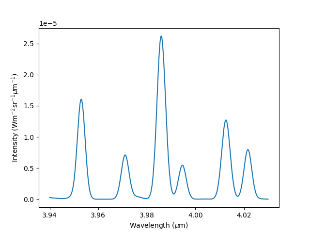
Neat, right?! We can now generate the spectrum for any temperature and density combination, with different wavelength coverage and at different spectral resolutions.
Real world (universe) examples
Below are a number of examples of how h3ppy can be applied to actual observations. The python code and the data are contained in the examples/ folder on the GitHub site.
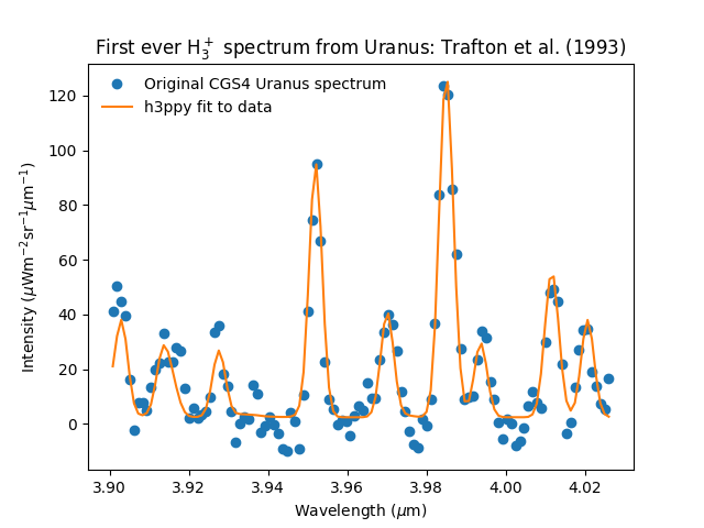
Example 1: UKIRT CGS4 Uranus spectrum
In our opinion, there are few spectra that are as historic as this one. It’s the first spectrum of \(\text{H}_3^+\) emission from Uranus and it was taken by Larry Trafton with the United Kingdom Infrared Telescope (UKIRT, now sadly defunct) in Hawai’i in 1992, and was published by Trafton et al. (1993, Astronomical Journal, 405, 761-766). The code and data for this example can be found here.
import matplotlib.pyplot as plt
import numpy as np
import h3ppy

# Read the UKIRT CGS4 data from Trafton et al., (1993)
data_file = 'cgs4_uranus_u01apr92.txt'
types = {'names' : ( 'w', 'i' ), 'formats' : ('f', 'f') }
dat = np.loadtxt(data_file, skiprows=4, dtype = types)

# Need to convert the instrument FOV to units of sterradian
# The pixel width is 3.1 arcsec with a slit widht of 3.1 arcsec
# Note - there are 4.2545e10 arceconds in a sterradian
spectrum = dat['i'] * 4.2545e10 / (3.1 * 3.1)
wave = dat['w']

# Make our h3ppy object :-)
h3p = h3ppy.h3p()

# Set the wavelength and data, and use the spectral resulution to input the
# expected line width
h3p.set(wavelength = wave, data = spectrum, R = 1300)

# We need to guess a temperature
h3p.set(temperature = 1000)

# Let h3ppy try and guess a wavelength offset
guess = h3p.guess_offset()

# Guess the density - this'll effectively scale the spectrum to the observed spectrum
# It really is not a measure of the actual density!
guess = h3p.guess_density()

# Let h3ppy do the fitting - this will do a full five parameter fit
fit = h3p.fit(verbose = False)

# Get the results
vars, errs = h3p.get_results()

# Plot the results!
fig, ax = plt.subplots()
ax.set_title('First ever H$_3^+$ spectrum from Uranus: Trafton et al. (1993)')
ax.plot(wave, spectrum * 1e6, 'o', label = 'Original CGS4 Uranus spectrum')
ax.plot(wave, fit * 1e6, label = 'h3ppy fit to data')
ax.legend(frameon = False)

# Use the h3ppy helper functions for the labels
ax.set_xlabel(h3p.xlabel())
ax.set_ylabel(h3p.ylabel(prefix = '$\mu$'))
plt.savefig('../img/cgs4_uranus_fit.png')
plt.close()
Which produces this fit:
and an output in the console of:
[h3ppy]  Spectrum parameters:
        Temperature    = 751.5 ± 42.7 [K]
        Column density = 1.23E+15 ± 2.73E+14 [m-2]
        ------------------------------
        sigma-0 = 1.63E-03 ± 6.49E-05
        offset-0 = -9.91E-04 ± 5.64E-05
        background-0 = 2.40E-06 ± 8.77E-07
which is very close to the published result, T = 740 K, that Trafton et al. (1992) got - yas! Also, note that h3ppy is using a \(\text{H}_3^+\) line list and partition function that weren’t available in 1992. This shows that h3ppy can reproduce past results, which is reassuring!
Example 2: Keck II NIRSPEC spectrum of Jupiter’s aurora
The twin Keck telescopes on Mauna Kea in Hawai’i are the largest optical telescopes in the world, and they have been used to observe \(\text{H}_3^+\) from the giant planets. Here, we will examine a spectrum of Jupiter’s southern aurora obtained with the NIRSPEC instrument. The code and data for this example can be found here.
NIRSPEC has a spectral resolution of \(R = \frac{\lambda}{\Delta \lambda} \sim 20,000\), which is sufficient to separate the \(\text{H}_3^+\) transition lines from each other. First we plot the data.
import matplotlib.pyplot as plt
import numpy as np
import h3ppy

# Read the Keck Jupiter data
data_file = 'nirspec_jupiter.txt'
types = {'names' : ( 'w', 'i' ), 'formats' : ('f', 'f') }
dat = np.loadtxt(data_file, skiprows=4, dtype = types)
wave = dat['w']
spec = dat['i']

# Create the h3ppy object feed data into it
h3p = h3ppy.h3p()

# Plot the observation
title = 'Keck NIRSPEC H$_3^+$ spectrum of the southern aurora of Jupiter'
fig, ax = plt.subplots()
ax.plot(wave, spec * 1e3)
ax.set(xlabel = h3p.xlabel(), ylabel = h3p.ylabel(prefix = 'm'), title = title)
plt.tight_layout()
plt.savefig('../img/nirspec_jupiter_data.png')
# plt.show()
plt.close()
Which produces this spectrum:
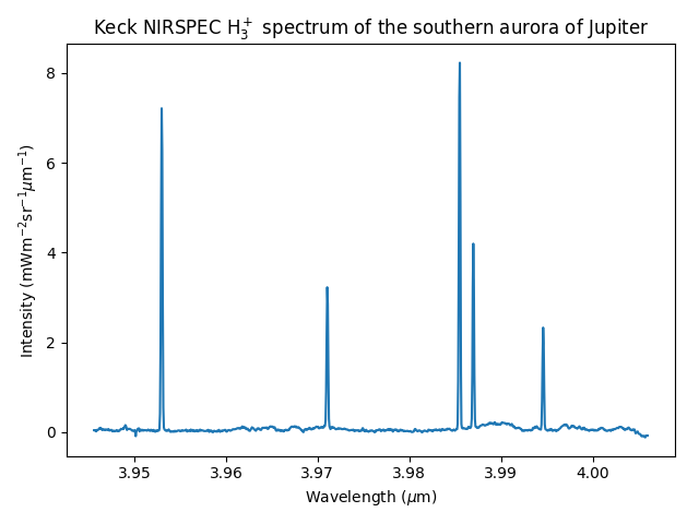
Since we are operating at a moderately high spectral resolution, I’m going to sub-divide the data, focusing on the individual spectral lines. This will not adversely affect the fit, since it is the relative intesity of the \(\text{H}_3^+\) spectral lines that determine the temperature and the density. By zooming into the plot above, I determine the approximate wavelength of the group of lines. The code below will reduce the wavelength range to focus only on the relevant \(\text{H}_3^+\) line regions, and then fit the resulting spectrum.
# This function sub-divides data centered on a list of wavelengths
def subdivide(wave, spec, middles, width = 20) :
ret = []
for m in middles :
centre = np.abs(wave - m).argmin()
for i in range(centre - width, centre + width) :
ret.append(spec[i])
return np.array(ret)
# The H3+ line centeres contained withing this spectral band
centers = [3.953, 3.971, 3.986, 3.9945]
cpos = np.arange(4) * 41 + 20
# Create sub-arrays, focusing on where the H3+ lines are
subspec = subdivide(wave, spec, centers)
subwave = subdivide(wave, wave, centers)
# Set the wavelength and the data
h3p.set(wavelength = subwave, data = subspec, R = 20000)
# Create a x scale for plotting
xx = range(len(subspec))
# Guess the density and proceed with a five parameter fit
h3p.guess_density()
fit = h3p.fit()
vars, errs = h3p.get_results()
# Plot the fit
fig, ax = plt.subplots()
ax.plot(xx, subspec * 1e3, '.', label = 'Observation')
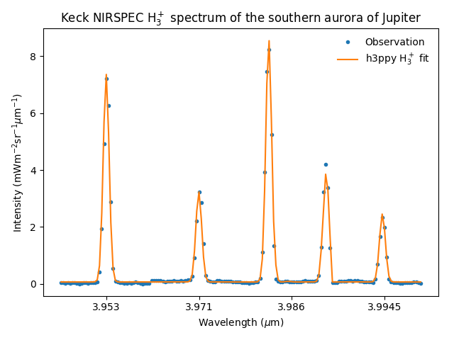
ax.plot(xx, fit * 1e3, label = 'h3ppy H$_3^+$ fit')
ax.set(xlabel = h3p.xlabel(), ylabel = h3p.ylabel(prefix = 'm'), xticks = cpos, title=title)
ax.set_xticklabels(centers)
ax.legend(frameon = False)
plt.tight_layout()
plt.savefig('../img/nirspec_jupiter_fit.png')
plt.close()
which produces a console output of
[h3ppy] Estimated density = 2.09E+15 m-2
[h3ppy]  Spectrum parameters:
        Temperature    = 923.6 ± 31.9 [K]
        Column density = 2.64E+15 ± 2.46E+14 [m-2]
        ------------------------------
        background-0 = 6.77E-05 ± 1.69E-05
        offset-0 = -1.46E-05 ± 1.13E-06
        sigma-0 = 7.82E-05 ± 1.17E-06
And looks like:
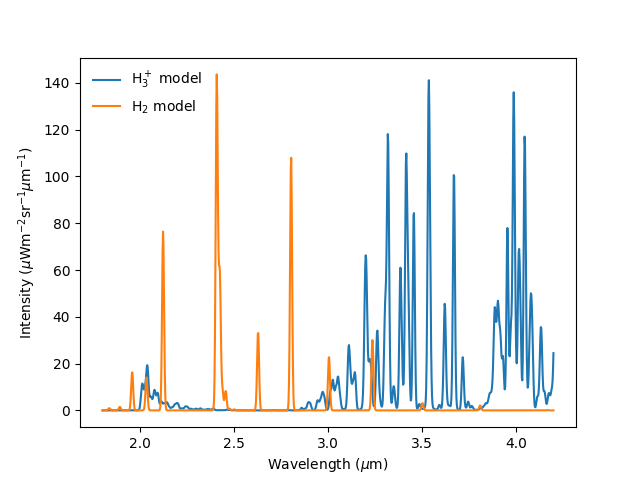
Example 3: Modelling the \(\text{H}_2\) spectrum
As of h3ppy version 0.3.0, there’s the functionality to model the quadropole \(\text{H}_2\) spectrum. The h2 class is functionally identical to the h3p class (it’s inherited from it), so works in the same way.
import h3ppy
import matplotlib.pyplot as plt
import numpy as np

# Instrument resolution
R = 300

# Temperature of the thermosphere
T = 900

# Set up the H3+ model
h3p = h3ppy.h3p()
h3p.set(temperature = T, density = 2e15, R = R)
wave = h3p.wavegen(1.8, 4.2, 1000)

# Set up the H2 model
amagat = 2.76e25
h2 = h3ppy.h2()
h2.set(temperature = T, density = amagat, R = R, wavelength = wave)

# Generate models
model_h3p = h3p.model()
model_h2  = h2.model()

# Plot the result
fig, ax = plt.subplots()
ax.plot(wave, model_h3p * 1e6, label = 'H$_3^+$ model')
ax.plot(wave, model_h2 * 1e6, label = 'H$_2$ model')
ax.set(ylabel = h3p.ylabel(prefix = '$\mu$'), xlabel = h3p.xlabel())
ax.legend(frameon = False)
plt.save('img/h2_h3p_spectrum.png')
``` Which looks like: