Basic Usage
Creating your first \(\text{H}_3^+\) model spectrum is easy.
import h3ppy

# Create the h3ppy H3+ object
h3p = h3ppy.h3p()

# Generate a wavelength scale (in microns)
wave = h3p.wavegen(3.4, 4.1, 1000)

# Set some physical parameters
# T - temperature
# N - Column density
# R - Spectral resolving power
# wave - wavelength scale
h3p.set(T = 1000, N = 1e16, R = 2700, wave = wave)

# Generate a model spectrum
m = h3p.model()
Take a look at the Examples for ways to use h3ppy.
Setting model parameters
The set(), model(), and fit() methods accepts the following inputs:
wavelength,wave,w- the wavelength scale on which to produce the model.data- the observed \(\text{H}_3^+\) spectrumtemperature,T- the intensity of the \(\text{H}_3^+\) spectral lines are an exponential function of the temperature. Typical ranges for the ionosphere’s of the giant planets are 400 (Saturn) to 1500 K (Jupiter).density,N- the column integrated \(\text{H}_3^+\) density, this is the number of ions along the line of sight vector. Typical ranges are \(10^{14} \text{ m}^{-2}\) (Neptune) up to \(10^{17} \text{ m}^{-2}\) (Jupiter).sigma_n- the n th polynomial constant of the spectral line width (sigma)offset_n- the n th polynomial constant of the wavelength offset from the rest wavelength. Doppler shift and wavelength calibration errors can offset the wavelength scale.background_n- the n th polynomial constant of the displacement from the zero radiace level of the spectrumnsigma- the number of polynomial constant used for the sigma.noffset- the number of polynomial constant used for the offset.nbackground- the number of polynomial constant used for the background.R- the spectral resolving power of the instrument. This is converted in the code to asigmaparameter.
Here we parameterise the width of the \(\text{H}_3^+\) lines with the sigma_n parameter. It is related to the full width of a line profile at half maximum (FWHM) by this expression:
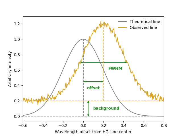
These paramters can be illustrated as follows (noting the relationship bewteeen the FWHM and sigma outlined above):
The parameters with _n suffix indicates that they are the n th polynomial constant (available for the offset, sigma, and background). For example, if we want use the following function to describe the sigma:
then we can tell h3ppy to use 3 polynomial constants:
h3p.set(nsigma = 3)
which is useful if you want to do some fitting. You can also specify the polynomial constants if you wish:
h3p.set(nsigma = 3, sigma_0 = 0.1, sigma_1 = 0.01, sigma_2 = 0.001)
Line lists and partition function
h3ppy uses \(\text{H}_3^+\) line data to produce models and fits from the following resources:
The \(\text{H}_3^+\) line list from Neale et al. (1996) - this data is available for download on the Exo Mol website.
The \(\text{H}_3^+\) partition function \(Q(T)\) and total emission \(E(T, N)\) from Miller et al. (2013).
The \(\text{H}_2\) line list and partition functioin from Roueff et al. (2019).